By Daniel Adler
The following article also appears on Huffington Post.
This summer, much was made of the end of Moneyball. The teams with the five highest win totals—the Yankees, Angels, Dodgers, Red Sox, Phillies—rank 1st, 6th, 9th, 4th, and 7th in opening day pay roll. Most of those teams took on even more salary during the season, so their final payroll ranks may even be higher.
After a few years of increasing parity in which we saw the A’s flourish, the Twins constantly competitive, the Marlins win a World Series, and even the Rays win the American League, disparity appeared to be on the rise this season. Harkening back to the late-1990s and the environment that spawned the Blue Ribbon Panel, this season seemed to be an extreme case of the haves versus the have-nots. The small market clubs who had recently feasted on undervalued players appear to have lost their competitive advantage since the big spenders started to buy into the same philosophies—in many cases hiring Ivy League stat geeks like ourselves. Michael Lewis’ concept of Moneyball was not about On-Base Percentage, but it was rather about finding undervalued assets. Was this the year the big market clubs finally started valuing assets correctly? Did money spent play a bigger role this season than in recent years? Intuition (and the Yankee World Series victory) says yes, but let’s take a look at the numbers.
Methodology
Looking at opening day payroll and wins, we test to see which seasons spending is the best predictor of wins. Since a team of replacement level players (e.g. talent available for the league minimum) could win 49 games, we will consider the number of games a team wins above 49 (marginal wins). Also, we will consider only the money spent above the minimum salary threshold (marginal dollars). This methodology, popularized by Baseball Prospectus is very common. Payroll data is courtesy of USA Today’s salary database.
Results
Running a simple regression trying to predict marginal wins as a function of marginal dollars spent, we will learn two things:
- Was marginal spending a significant (i.e. non-random predictor) of marginal wins? This is the p-value. The p-value represents the percent chance that the predictor is random. If the p-value is .50, that means there was a 50% chance it is random (spending does not impact wins). Lower p-value means spending was more important.
- What percentage of variation in marginal wins can we predict if we know spending? This is called the r2. A high r2 means that we can predict more of the variation in wins based on spending. If r2 were .05, that would mean we could predict 5% of the variance in wins if we knew spending. For r2, higher means money spent was a greater predictor of wins.
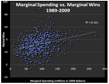
First, let’s run a quick regression looking at all years since 1989. To account for payroll inflation, I have brought everything up to present value using a discount rate of 8% (the average rate of inflation in recent seasons).

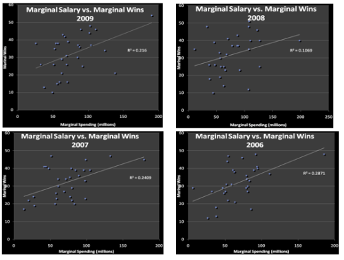
Unsurprisingly, over the past 20 years, opening day marginal salary has been a significant predictor of wins. This estimate is not very precise since the 8% discount rate is an approximation and just allows us to consider all years on the same graph. We will get a clearer picture looking at each season individually.

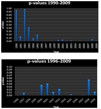
As you can see, in the early 1990s, salary did not predict wins for many of the years (high p-values). However, considering the full seasons after the strike, we see that salary has always been a good predictor (with 2008 being the only year p>.05).
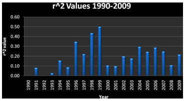
This is where things get interesting. In the years leading up to the strike (1990-1993), salary was a poor predictor of marginal wins. Immediately after the strike, there was a series of years in which marginal salary was a good predictor of marginal wins. This is when parity hit its nadir and the Blue Ribbon panel was ordered. In 2000 and 2001 (both years in which the Yankees made the World Series), money was a very poor predictor of wins. Since then, the r2 has hovered in the .17-.29 range, with 2008 (the year of the Rays) being a notable outlier at .107.
Considering the past 8 seasons, this year was not particularly notable in terms of payroll predicting success. However, the big market clubs are spending smarter, particularly in the draft and on Latin American teenagers, which is not reflected in opening day payrolls. The margin for error for the little guys is razor thin and the window of opportunity can be very short (see: Indians’ downfall after 2007 and Rays’ slide after 2008). However, the data suggest that this year may not have called for the alarmist musings by some members of the media. Competitive balance is probably not what it should be, but this year was hardly different from most other recent seasons.

Very nice analysis. The very low payroll-wins correlation prior to 1994 is very interesting. Do you have any data that would allow you to look at earlier years, to see if this was just a short-term drop or whether it was generally true prior to 2004?
I would generally caution against drawing the conclusion, based on one year correlations, that the payroll-wins link is weak. Because most teams are fairly tightly clustered in payroll, and the SD of win% in baseball is very low (i.e. very competitive), the correlation will be fairly low even if teams were perfectly identifying the value of talent. Random variation in performance plus injuries would probably limit the r to something like .6.
If you pool seasons, you can see that the payroll-wins relationship is very strong. Tango did this for 1998-2009, and found an r of .75. Over a several year period, the advantage of spending more is clear and large: http://www.insidethebook.com/ee/index.php/site/comments/how_many_wins_are_those_dollars_buying/.
And what we really care about most, I think, is whether payroll determines which teams make the post-season. And the link there has been very strong. A while back I looked at data from 1992-2005, including hypothetical wildcards for 1992-1993 (I only gave 1 WC slot to the 12-team 1992 NL), I get the following results. For each payroll quintile, this is the number of championships/wildcards a team won per decade:
Top 4.9
2nd 3.0
3rd 2.4
4th 1.8
5th 1.2
So a top-quintile team can expect to reach the postseason 4x as often as a bottom-quintile team. (Or, fans of rich teams have to endure one non-playoff year between championships, on average, while poor teams have to endure 7.) Whatever your r2 shows, I think fans would tell you that is a big difference.